Numpy.convolve() method calculates the discrete, linear convolution of two one-dimensional sequences (arrays).

Convolution is a mathematical operation that combines two signals to produce a third signal, representing how one modifies the other. In layman’s terms, it “slides” one array (the kernel/filter) over another and calculates the sum of elementwise products at each position.

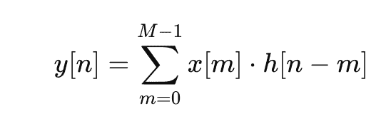
Mathematically, convolution is defined as:

Let’s apply a kernel to smooth a signal.

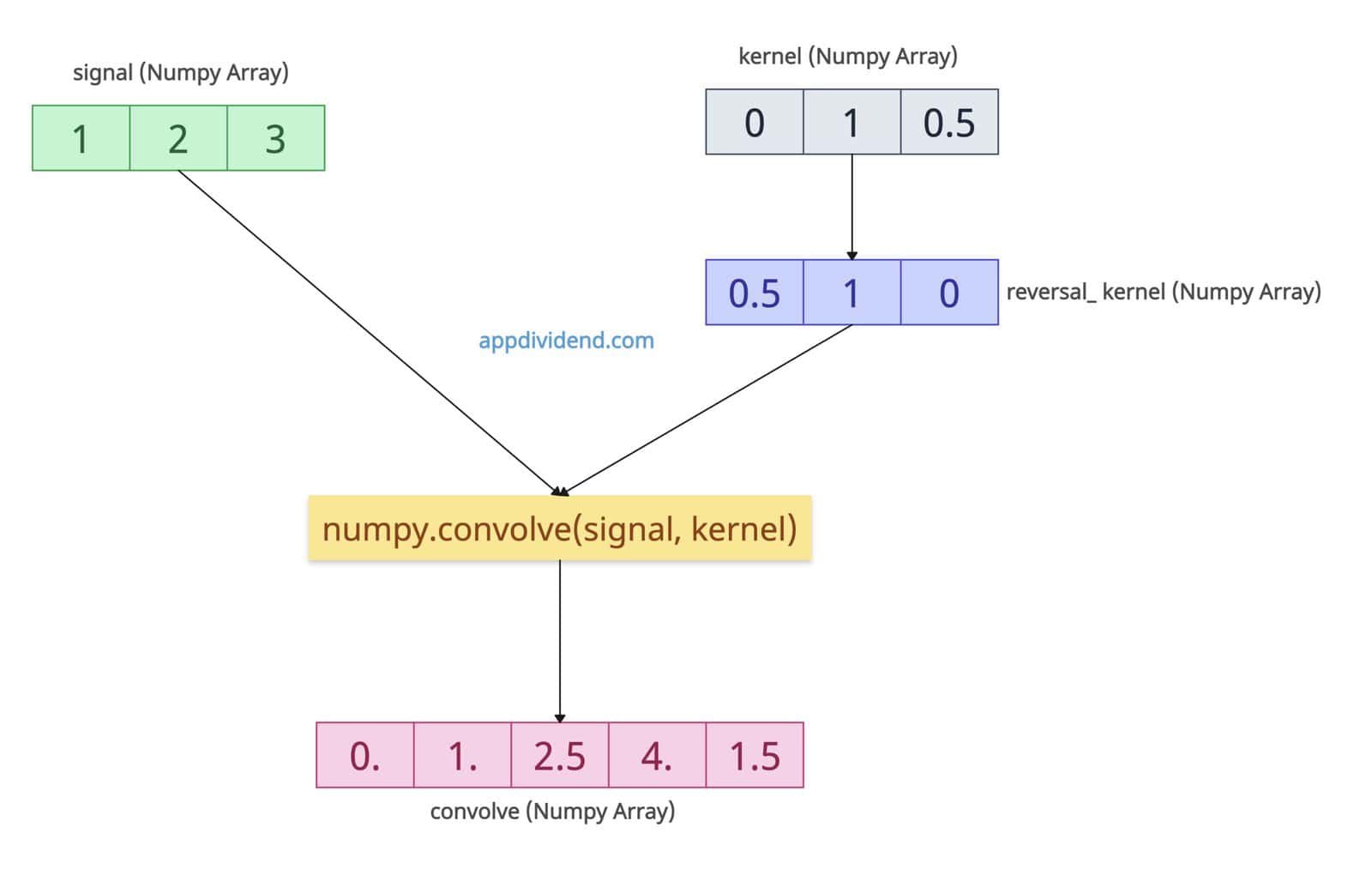
import numpy as np

signal = np.array([1, 2, 3])

kernel = np.array([0, 1, 0.5])

convolve = np.convolve(signal, kernel)

print(convolve)

# Output: [0.  1.  2.5   4.  1.5]

In this code, you can think of a signal as the primary data that represents the input sequence. The “kernel” (also referred to as a filter or window) is what slides over the signal.

Since we have not specified a mode, by default, it considers the mode=”full” and performs the full linear convolution of these two 1D arrays.

Now, before convolution, the kernel is flipped or reversed.

kernel = [0, 1, 0.5]  →  reversed_kernel = [0.5, 1, 0]

Therefore, when performing calculations, we need to use the reversed_kernel values instead of the input kernel values. It slides the reversed kernel across the signal and calculates the sum of elementwise products at each step.

Now, our input signal is this: [1, 2, 3]

The reversed_kernel is this: [0.5, 1, 0].

Step	Overlap	Calculation	Output
1	[1] × [0]	1×0 = 0	0.0
2	[1,2] × [1,0]	1×1 + 2×0 = 1	1.0
3	[1,2,3] × [0.5,1,0]	0.5 + 2 + 0 = 2.5	2.5
4	[2,3] × [0.5,1]	1 + 3 = 4	4.0
5	[3] × [0.5]	1.5	1.5

The output represents the full linear convolution, and you can calculate its length using this formula:

length = len(signal) + len(kernel) – 1 = 5.

Syntax

numpy.convolve(arr, v, mode='full')

Parameters

Argument	Description
arr (array_like)	It represents the input array (signal).
v (array_like)	It represents the second array (filter or kernel)
mode {‘full’, ‘valid’, ‘same’}	It defines the size of an input array. “full”: This is the default mode, which returns the full discrete linear convolution. “same”: It returns the output array, which is of the same size as an input array (centered). “valid”: It returns only parts where both arrays fully overlap.

Mode variations

mode=”same”

It maintains the input length for filtering. It only keeps the middle 3 values, aligning the kernel roughly in the center of the signal.

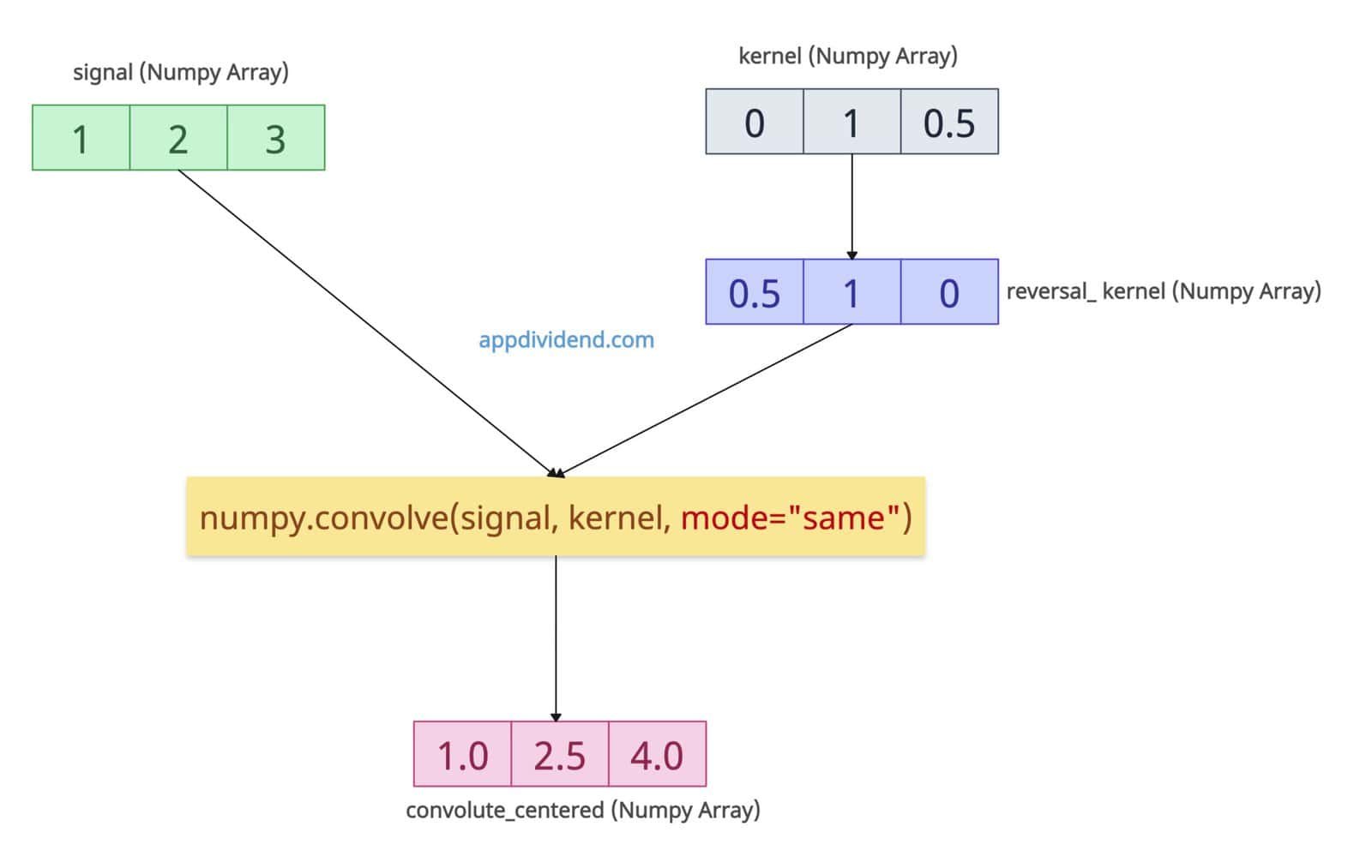
import numpy as np

signal = np.array([1, 2, 3])

kernel = np.array([0, 1, 0.5])

convolute_centered = np.convolve(signal, kernel, mode="same")

print(convolute_centered)

# Output: [1.  2.5 4. ]

You can see that the output array has the same length as the input signal.

Center Position	Overlap	Multiplication	Output
Over 1	[1, 2] × [1, 0]	(1×1) + (2×0) = 1	1.0
Over 2	[1, 2, 3] × [0.5, 1, 0]	(1×0.5) + (2×1) + (3×0) = 0.5 + 2 = 2.5	2.5
Over 3	[2, 3] × [0.5, 1]	(2×0.5) + (3×1) = 1 + 3 = 4	4.0

mode=”valid”

It represents the smallest overlap (requires full filter coverage).

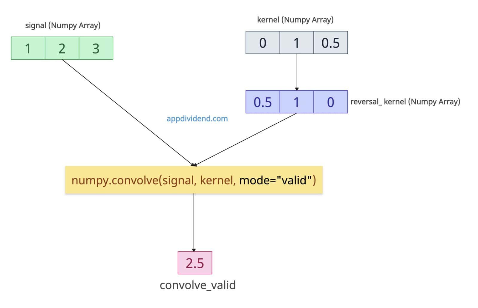
import numpy as np

signal = np.array([1, 2, 3])

kernel = np.array([0, 1, 0.5])

convolve_valid = np.convolve(signal, kernel, mode="valid")

print(convolve_valid)

# Output: [2.5]

For ‘valid’, both arrays must completely overlap.

output length = len(signal) − len(kernel) + 1 = 3 − 3 + 1 = 1.

So there’s exactly one position where the kernel fully overlaps the signal, and that is the centered position.

Signal	Kernel (reversed)	Elementwise Multiplication	Sum